Back in the Trenches, Part 1: Karaul!

Dedicated to the Department of Applied Mathematics at Altai State Technical University.

Especially to Semion Kantor – “your brains must be boiling!” was his way of saying get to work. And it worked. To Elena Kryuchkova and Larisa Suchkova, who could read your code written on a piece of paper – LISP, C++, it didn’t matter – and immediately name the edge condition under which it would fail. No IDE required, no compiler, just the kind of deep intuition that only forms through years of looking at how minds make mistakes. The pruning bug in this article would not have survived their review.

“Пока противник рисует карты наступления, мы меняем ландшафты, причём вручную. Когда приходит время атаки, противник теряется на незнакомой местности и приходит в полную небоеготовность. В этом смысл, в этом наша стратегия.” (с) к/ф “ДМБ”, 2000

“While the enemy draws maps of the offensive, we change the landscapes – manually. When the time to attack comes, the enemy gets lost in unfamiliar terrain and becomes completely combat-ineffective. That is the meaning, that is our strategy.” – DMB, 2000

Карау́л

The moment I decided to integrate anomaly detection into our call volume monitoring, I discovered that Microsoft was sunsetting its Anomaly Detector service. The notice was buried in a changelog, the way these things always are – matter-of-fact, with a migration guide pointing to alternatives and a timeline that feels generous until you actually read it. I’ve seen this movie before with enough platforms to know how it ends.

Most CIOs would start a procurement process, evaluate vendors, raise a PO, and have something running by Q2 < year unknown >. I opened VS Code.

For the impatient: GitHub

Aperture Science: we do what we must because we can. – GLaDOS, Portal

This wasn’t recklessness – it was a deliberate choice that connects directly to everything I’ve been writing about in this series. In Zen and the Art of Making Samogon I argued that engineering intuition atrophies when you stop touching the machine. In the TRIZ and DT series, Part 1 Triz and DT, Part 2  I showed how first principles thinking produces solutions that a vendor catalog will never contain. This article is both of those ideas applied to a real business problem, in real TypeScript, with real data, and with the very real suffering that comes from implementing a pruning algorithm when you have an early leadership call the next morning.

The result is karaul – a TypeScript changepoint detection library. The name carries two meanings and I chose both of them deliberately. In Russian, karaul (карау́л) means guard duty – a sentinel, something that stands watch over your data in silence, looking for the moment something permanently shifts. But Карау́л! is also what Russians shout when everything goes sideways – the alarm, the exclamation, the signal that the situation has changed and someone needs to pay attention right now. A system that stands watch quietly and screams when the data breaks seemed to deserve a name that does both.

I lead the technology organization for the Americas region at Align Technology – the company behind Invisalign. And last week I spent an embarrassing amount of time at night debugging a pruning condition that turned out to hinge on a single character – <= versus < – in a filter predicate. Both things are true, and I wouldn’t change either of them. Engineering leaders who stop getting their hands dirty eventually stop understanding what their teams are actually doing – and that gap, in my experience, is where the most expensive mistakes hide.

So join me in this adventure. What follows covers algorithms, mathematics, dynamic programming, complexity theory, statistics, object oriented design patterns, and TypeScript – not as a structured curriculum but as an honest account of what it looks like when a CIO goes back to first principles and builds something from scratch instead of raising a PO. A personal CS50, if you will, written in a traffic jam on Marginal Pinheiros in the São Paulo Easter rain, between boxing sessions and leadership calls.

The suffering, I promise, is the point.

The Signal Behind The Noise

Call volume is one of those metrics that lives on every customer support dashboard and gets genuinely understood by almost nobody. It goes up, it goes down, someone adds it to a weekly report, and the conversation usually ends there. Which is a shame, because if you know how to read it, call volume is one of the most honest signals a business produces.

When customers call, something happened. Maybe your product confused them, maybe your last deployment broke something subtle, maybe you delivered something genuinely good and now everyone wants more of it. The call is the symptom. The volume shift is the pattern. And the moment that pattern permanently changes – not a spike, not noise, but a sustained structural shift in behavior – something in your business changed with it.

That’s the distinction that matters. A spike on a Monday after a weekend outage is expected and boring. A sustained 40% increase in call volume starting the day after a deployment and not returning to baseline two weeks later – that’s a signal worth understanding. Not because the number went up, but because something in the relationship between your product and your customers shifted, and it hasn’t shifted back.

We deliver things constantly – features, fixes, process changes, pricing updates. Some land well. Some don’t. The honest feedback rarely comes from surveys or NPS scores, which customers fill out when they’re either delighted or furious and almost never in between. It comes from the calls. From the words customers use when they’re confused, frustrated, or genuinely trying to understand something that should have been obvious. The volume tells you when something changed. The transcripts tell you what it felt like from the other side.

This is where the connection to Design Thinking becomes concrete rather than theoretical. The classic DT empathy phase says go talk to your customers – schedule interviews, run focus groups, synthesize findings over several weeks. We are already talking to them. Every call is a conversation. Every transcript is an empathy interview that happened whether you planned it or not. The question is whether you’re listening systematically or letting it pile up in a storage bucket as a compliance artifact.

karaul is the listening layer. It watches the signal, detects when something has permanently shifted, and hands you a timestamp. Everything else – the transcripts, the Jira tickets, the deployment notes, the LLM reasoning over all of it – flows from that timestamp. But none of it is useful without first knowing precisely when the shit shift happened.

So What Exactly Is A Changepoint

Before reaching for a tool – any tool – it helps to understand the problem precisely. A changepoint is the moment when the statistical behavior of a time series permanently shifts. Not a spike, not noise, not the predictable end-of-month surge that your business runs like clockwork – cyclic patterns that return to baseline are expected behavior, not structural shifts. A changepoint is a permanent shift – a new baseline that doesn’t return to the previous one.

The Nile river is the canonical example in the literature. Annual flow volume measured at Aswan from 1871 to 1970 – a hundred years of data, one changepoint at 1899, when construction of the first Aswan dam was underway and the hydrology of the river changed permanently. The data knew before the history books confirmed it. That is what a changepoint detector does – it finds the moment the underlying process changed, not just the moment the number moved.

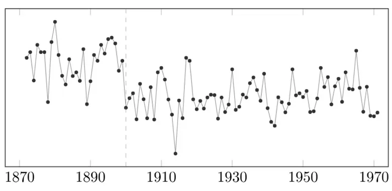
By van den Burg, Gerrit JJ, and Christopher KI Williams. - van den Burg, Gerrit JJ, and Christopher KI Williams. “An Evaluation of Change Point Detection Algorithms.” arXiv preprint arXiv:2003.06222 (2020)., CC BY-SA 4.0, https://commons.wikimedia.org/w/index.php?curid=91477629

In your call volume data the equivalent is the day after a deployment that introduced a confusing billing flow, or the week a new product feature generated more questions than it answered, or the moment a process change permanently altered the baseline. The number moved and stayed moved. Something changed.

Formally, the problem is to find the optimal set of split points that partition your time series into segments, where each segment is statistically homogeneous – meaning the variation within it is just noise around a stable mean – while minimizing a cost function penalized by the number of splits. The mathematics behind this are not trivial. The original Killick et al. 2012 paper is on arxiv – dense, rigorous, full of **argmax **notation that is not pirate speak, and worth every minute if you have a healthy relationship with double integrals and measure theory. For everyone else, I will cover the intuition here and enough of the mathematics to implement it correctly.

The Temptation

I have watched this pattern repeat across my entire career, and it always starts the same way.

In the early 2000s, Delphi was having its moment – a vast component ecosystem where you could drag a neural network onto a form, set a few properties, and ship by Friday with zero understanding of backpropagation, activation functions, or gradient descent. The community was generous, the components worked mostly, and the gap between what you could ship and what you actually understood grew quietly in the background until it didn’t.

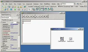
pip install is the new drag and drop. The ecosystem is larger, the abstractions are more powerful, and the gap has never been wider. This is not a criticism – open source is one of the great gifts of our industry. It is an observation about what happens to engineering intuition when convenience becomes the default and first principles become optional. You will skip the off-by-one errors in the DP table. You will skip the pruning condition that took an embarrassing amount of time to get right. You will skip the moment when the Gaussian cost function finally makes sense not as a formula but as an idea. And you will ship faster, and understand less, and the next time something breaks in production you will have fewer tools to reason about why.

New neural pathways form through struggle, not through abstraction. This is not nostalgia for difficulty – it is an observation about how deep understanding actually develops. The Strugatsky brothers, who understood human nature rather better than most, put it this way in a slightly different context:

“Общение с девушками доставляет удовольствие лишь в тех случаях, когда достигается через преодоление препятствий.”

– Аркадий и Борис Стругацкие, *Понедельник начинается в субботу *(1964)

“The pursuit of young ladies only brings satisfaction when it involves overcoming obstacles.”

– Arkady and Boris Strugatsky, Monday Starts on Saturday (1964)

The principle generalizes further than they probably intended.

When You Have A Hammer

There is a rhetorical pattern I encounter with increasing frequency in technology leadership conversations, and it goes roughly like this: whatever the problem, whatever the context, whatever the constraints – just use AI for it. The confidence with which this is said is inversely proportional to the specificity of what “it” actually is. It is a mystical belief dressed in the language of pragmatism, and it is the most recent incarnation of a very old engineering mistake.

I have seen this before. When genetic algorithms became accessible in the late 1990s, a generation of engineers discovered that you could frame almost any optimization problem as a search over a solution space, define a fitness function, and let evolution do the work. The abstraction was genuinely elegant – and genuinely seductive. Suddenly every problem looked like an optimization landscape.

I used genetic algorithms for sales representative route optimization in production. It produced routes. Whether those routes were optimal is a question I prefer not to investigate too closely – a few sales reps may have had opinions, but they were not particularly forthcoming with structured feedback, and the plural of anecdote is not data. We shall call it a learning experience and move on.

Later in this article you will see exactly how tempting it is to reach for GA when building a changepoint detector. The parallel to today’s AI moment is not accidental – same seduction mechanism, different decade. When you have a hammer with a very impressive handle, everything starts looking like a nail. The question worth asking – every time, for every tool – is not whether it can do this, but whether it is the right thing for this.

Building Karaul – From First Principles

Start With A Test

Before writing a single line of implementation, we need something to validate against. The Turing Change Point Dataset (TCPD), maintained by the Alan Turing Institute and available on GitHub, is the standard benchmark for changepoint detection algorithms – 37 real-world time series, each annotated by five human experts with known ground truth changepoint locations.

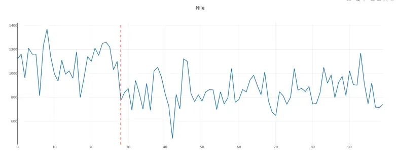
The Nile dataset is the simplest entry – 100 years of annual flow volume at Aswan, one known changepoint at 1899. Index 28 in the data. The detector that can’t find this has no business in production.

function testNile() {
    const nile = loadTCPD('./fixtures/nile.json');
    const changepoints = pelt(nile, estimatePenalty(nile));

    console.assert(changepoints.length === 1, 'Expected one changepoint');
    console.assert(changepoints[0] === 28, 'Expected changepoint at index 28 (year 1899)');

    console.log('Nile test passed:', changepoints);
}

A proper test suite using Vitest – TypeScript’s natural testing framework for ESM projects – is a natural next step and left as an exercise.

The Naive Solution and Why It Will Kill You In Production

The brute force approach to finding changepoints is conceptually simple: enumerate every possible combination of split points, compute the cost of each segmentation, return the minimum. For a series of n points there are n-1 possible split positions. Each is either a changepoint or not – a binary choice. Total combinations: 2ⁿ⁻¹.

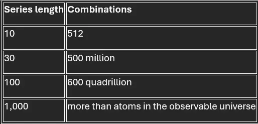
Your call volume series might have tens of thousands of points. Brute force is not slow – it is physically impossible.

This is the moment to talk about algorithmic complexity, briefly and honestly. O(n²) means that doubling your data quadruples your runtime. O(2ⁿ) means adding one data point doubles it. These are not academic distinctions – they are the difference between a system that scales and one that becomes your 3am incident. I have watched teams demo flawlessly on a thousand rows and collapse completely on a million, consistently surprised that the thing that worked in testing does not work in production. The dataset size changed. The complexity did not.

The correct algorithm – PELT, Pruned Exact Linear Time, introduced by Killick, Fearnhead and Eckley in 2012 – solves this exactly and efficiently. Feeling adventurous to dive deep into the math? https://arxiv.org/abs/1101.1438

Dynamic Programming – The Key Insight

The reason PELT is efficient is dynamic programming – a technique for solving problems by breaking them into overlapping subproblems, solving each once, and storing the result so you never recompute it.

The natural way to think about optimal segmentation is recursive:

“What is the cheapest way to segment the series up to point t?”

F(t) = min over all s < t of: F(s) + C(s, t) + β

F(t) is the optimal cost of segmenting everything up to point t. C(s, t) is the cost of the segment from s to t. β is the penalty – a tax on complexity that prevents the algorithm from splitting every point into its own segment. To find F(t) you try every possible last changepoint s, building on F(s) which you already computed. No redundant computation. F(0) = 0 by definition – the cost of segmenting nothing is zero.

The recursive implementation maps directly to the formula – clean, readable, and wrong for production:

// Top-down: elegant, intuitive, and will overflow your stack on real data
const memo = new Map<number, number>();

function F(t: number): number {
    if (t === 0) return 0;

    if (memo.has(t)) return memo.get(t)!;

    let best = Infinity;
    for (let s = 0; s < t; s++) {
        best = Math.min(best, F(s) + computeCost(series, s, t) + penalty);
    }

    memo.set(t, best);

    return best;
}
// Call it: F(n) – starts from the top, recurses down

The bottom-up version computes the same recurrence but fills the table iteratively from F(0) upward. No recursion, no stack risk, no repeated function calls – just a loop and an array:

// Bottom-up: fills the table forward, builds on what it already knows

const F = new Array(n + 1).fill(Infinity);

F[0] = 0;

for (let t = 1; t <= n; t++) {
    for (let s = 0; s < t; s++) {
        const cost = F[s] + computeCost(series, s, t) + penalty;

        if (cost < F[t]) {
            F[t] = cost;
            cps[t] = s; // record where the optimal split was
        }
    }
}
// F[n] now contains the optimal total cost
// cps[] contains the breadcrumb trail for traceback

The result is identical. The difference is execution – top-down computes on demand and risks stack overflow on long series, bottom-up computes everything in order and keeps memory flat. For a time series with thousands of points there is no real choice. The recursive version is here because it shows you what the algorithm is. The iterative version is what you actually ship.

The penalty β deserves a moment. Without it the algorithm splits every point into its own segment – zero variance, zero cost, technically perfect, completely useless – like a performance review that gives everyone a ten out of ten. The penalty makes each split justify itself: a changepoint is only added if it reduces total cost by more than β. Low penalty – sensitive, finds many changepoints. High penalty – conservative, finds only the most dramatic shifts. We will automate this choice shortly and spare you the manual tuning that makes grown engineers cry.

The Cost Function – And A Tempting Detour

The cost function C(s, t) measures how well a single statistical model explains the data in a segment. For detecting mean shifts in call volume we use the Gaussian cost, which assumes data within each segment is drawn from a normal distribution and measures how much variance exists within it. From maximum likelihood estimation, dropping constants that cancel across segments:

C(s, t) = n · log(σ²)

Where n is the segment length and σ² is the sample variance. A segment of constant values has zero variance, zero cost – perfect fit. A segment spanning two different means has high variance, high cost – it should be split. The intuition is simple even if the derivation involves the kind of notation that makes non-mathematicians question their life choices.

Now look at the cost function for a moment. It takes a segment and returns a number measuring how well a model fits it. It penalizes heterogeneity. It rewards homogeneity. That is a fitness function.

And this is where it gets interesting – or dangerous, depending on how you look at it. When I first discovered genetic algorithms alongside C++ templates, generics, and operator overloading, it felt like someone had handed me a universal key. The revelation was genuine: you could express almost any optimization problem in three methods, plug it into a framework, and let evolution do the thinking. Define what “good” looks like, define how solutions combine and mutate, and the algorithm searches the space for you. The abstraction was so clean it felt like cheating.

For changepoint detection the template practically writes itself. A segmentation is a binary chromosome – each bit a potential split. Fitness is negative total segment cost. Crossover splices two segmentations at a random point. Mutation flips a bit. In C++ with operator overloading, crossover can literally look like addition:

template <typename T>

class GeneticAlgorithm {
public:
    virtual T crossover(T parent1, T parent2) = 0;
    virtual T mutate(T candidate) = 0;
    virtual double fitness(T candidate) = 0;

    T solve(std::vector<T> population) {
        // evolution handles the rest
    }
};
 
// crossover looks like addition – elegant, seductive, slightly unhinged
Segmentation operator+(Segmentation& a, Segmentation& b) {
    return crossover(a, b);
}

Done. Ship it. Call it innovation.

Detour – The Lazy Engineer’s Revelation

To be fair to my younger self and to the algorithm – GA for changepoint detection is not completely wrong. There are published papers exploring exactly this, and for problems with complex non-decomposable cost functions where exact methods don’t exist, a well-tuned GA can be a legitimate choice. The universe is large and nuanced.

For our problem specifically the argument is precise. PELT finds the globally optimal segmentation, deterministically, every single time. GA finds a good-enough segmentation, approximately, differently each run, with no mathematical guarantee about how far from optimal it landed. That gap – between “probably fine” and “provably correct” – matters enormously when you are making business decisions based on the output.

The reason GA feels so natural here is the same reason LLMs feel natural for almost everything right now. Both are powerful general frameworks that abstract away the hard thinking. Both are deceptively easy to apply – define a fitness function, write a prompt, something comes out the other end and it looks like an answer. The implementation effort is low. The intellectual effort of asking whether this is actually the right tool is higher, less immediately rewarding, and distressingly easy to skip. When you have a hammer with a very impressive handle and an enthusiastic community writing papers about all the nails it can hit, the temptation is real and the consequences are subtle enough that you might not notice them until a sales rep is driving in circles.

PELT is not more impressive than GA. It is more correct for this problem. That distinction is the whole point.

The Strategy Pattern – OOP Done Right

The Gaussian model assumes normally distributed noise – reasonable for many signals. For count data like call volumes, which are non-negative integers, a Poisson cost function is theoretically more appropriate. PELT doesn’t care which model you use. It only needs something that takes a segment and returns a number.

This is the Strategy pattern – one of the foundational patterns from the Gang of Four’s *Design Patterns *https://en.wikipedia.org/wiki/Design_Patterns, published in 1994 and still worth reading thirty years later. Define an interface for the behavior that varies, implement it differently for each case, let the algorithm work with the interface rather than any specific implementation.

interface CostFunction {
    compute(series: TimeSeries, start: number, end: number): number;
}
class GaussianCost implements CostFunction {
    compute(series: TimeSeries, start: number, end: number): number {
        // n · log(σ²)
    }
}
class PoissonCost implements CostFunction {
    compute(series: TimeSeries, start: number, end: number): number {
        // different model, same interface
    }
}

This is polymorphism in practice – not the textbook Animal class that barks or meows depending on runtime type, but a real abstraction where the same algorithm produces different behavior depending on which cost function you hand it. Gaussian today, Poisson tomorrow, something you invent next week. The word sounds like a disease. The concept is one of the more powerful ideas in software engineering, and the C++ template from the GA detour above is its slightly feverish cousin – same family, different disposition.

The current karaul implementation uses Gaussian cost directly – the CostFunction interface is noted as a TODO, deferred until there are two concrete implementations to generalize from. Premature abstraction is the structural equivalent of premature optimization. Don’t abstract until you feel the pain.

Pruning – The P in PELT

The DP above is O(n²) – for every point t you examine all previous candidates s. Better than brute force, but still quadratic. For 10,000 points that is 100 million operations, and for 100,000 it is 10 billion – territory where your users start composing strongly worded emails.

PELT adds one insight: if a candidate s is already worse than the current best at time t, and the cost function only grows as segments get longer, then s can never be optimal for any future point either. Discard it permanently. The active candidate set shrinks over time, and with it the work at each step.

The core DP loop with pruning:

for (let t = 1; t <= n; t++) {
    for (const s of active) {
        const cost = F[s] + computeCost(series, s, t) + penalty;
        if (cost < F[t]) {
            F[t] = cost;
            cps[t] = s;
        }
    }

//TODO: this can be optimizied further, also computeCost is computed unnecessarily here
    active = active.filter(s => F[s] + computeCost(series, s, t) <= F[t]);
    active.push(t);
}

The order matters precisely: compute F[t] first, prune second, add current point third. The condition is <= not <. These details are not obvious and the consequences of getting them wrong are exactly the kind of bug that passes all your small dataset tests and only surfaces when the data gets real – at which point you will have already presented the results to leadership with considerable confidence.

A note for the fastidious: Array.filter creates a new array on every iteration, giving the garbage collector unnecessary work at scale. The correct approach is in-place removal – iterating backwards and splicing, or maintaining the active set as a more appropriate data structure. This is left as an exercise, and also as a reminder that premature optimization is the root of all evil – Knuth said it, he meant it, and the readable version ships first. Make it work, make it right, make it fast – in that order, with appropriate guilt at each transition.

Implementing the pruning condition correctly was harder than I expected – like deciding to carry these home on foot instead of taking a taxi. I could have used an existing library, of course. Skipped the off-by-one errors, skipped the <= vs < existential crisis, skipped the part where I sat quietly with my own hubris and a failing test suite. Remember the point about suffering and struggle? One time carrying didn’t make me stronger. But it made me smarter about estimating my limits – which, when you think about it, is the more durable improvement. Stronger fades. Smarter compounds.

Traceback – Finding The Changepoints

The DP loop fills the F table and records in cps[t] the optimal last split point for each position. To recover the actual changepoint locations you walk backwards from the end, following the breadcrumb trail:

let t = n;
while (t > 0) {
    const s = cps[t];
    if (s > 0) result.push(s);
    t = s;
}
return result.reverse();

cps[n] tells you where the last segment started. That position’s cps entry tells you where the segment before it started. And so on, back to zero. Reverse the collected positions and you have your changepoints in chronological order. The entire algorithm – DP, pruning, traceback – is roughly 25 lines of TypeScript. The mathematics behind it took decades to develop. This ratio feels about right.

Automatic Penalty Selection

Manually tuning β is not a production solution – it works beautifully in a controlled environment and falls apart spectacularly the moment someone runs it on a dataset you hadn’t considered, ideally right before a release, preferably in production.

estimatePenalty derives the penalty directly from the data. It computes first differences –absolute changes between consecutive values – and takes their median absolute difference. Because first differences of Gaussian noise scale as σ√2, the result is divided by 0.6745 × √2 ≈ 0.9534 to recover σ, the within-segment noise level.

export function estimatePenalty(series: TimeSeries): number {
    const n = series.length;

    const differences = series
        .slice(1)
        .map((val, i) => Math.abs(val - series[i]!));

    const sorted = [...differences].sort((a, b) => a - b);

    // 0.9534 = 0.6745 * sqrt(2) -- correct MAD divisor for first differences
    const MAD = median(sorted, true);
    const sigma = MAD / (0.6745 * Math.sqrt(2));

    // floor at 1 prevents negative penalty when sigma < 1
    const logSigma2 = Math.log(Math.max(sigma ** 2, 1));

    return Math.log(n) * logSigma2;
}

The penalty is log(n) · log(σ²). The log(n) term is the Bayesian Information Criterion (BIC) scaling factor – it grows with series length to guard against overfitting as more split opportunities arise. The log(σ²) term matches the scale of the Gaussian cost function, which operates in log-variance space, making the penalty self-calibrating: louder series automatically get a larger penalty, quieter ones a smaller one. The floor at max(σ², 1) prevents negative penalties on normalized or low-amplitude series, which would otherwise incentivize PELT to split every point.

If automatic selection doesn’t suit your data, pelt(series, penalty) accepts a manual penalty directly.

Does It Work

Two validation cases.

The Nile dataset – karaul finds the 1899 changepoint exactly, with automatic penalty selection, every time. The beginning of Aswan dam construction shows up in the data 125 years later. This is what correct looks like.

Synthetic call volume – 365 days simulating a realistic operational environment: biweekly deployments shifting the baseline by varying amounts, layered with predictable month-end volume spikes. Twelve changepoints are planted at every 14-day deployment boundary. karaul finds all twelve. The month-end spikes are correctly ignored – cyclic patterns that return to baseline are not structural shifts, and the algorithm is right to treat them that way.

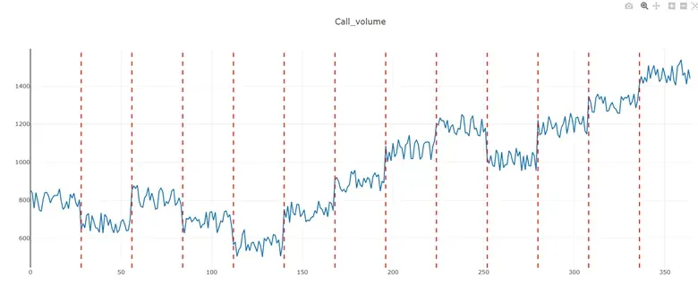
The full implementation is on GitHub. The suffering is included at no extra charge.

What Comes Next

karaul is standing watch. It knows when your call volume has permanently shifted. It knows when your baseline changed, when something in your business moved and didn’t move back. What it doesn’t know – and what no algorithm can tell you – is why.

That is a different problem. It requires reading transcripts, correlating deployments, reasoning over context, and connecting the signal to human experience. It requires Design Thinking without the research sprint, because the research sprint already happened – every time a customer picked up the phone.

In Part 2 we take karaul into production. Twilio, call transcripts, Jira tickets, and an LLM doing exactly one thing – the one thing it is actually built for. The pipeline closes. The sentinel stops watching and starts talking.

This was a triumph

I’m making a note here: huge success

It’s hard to overstate my satisfaction Aperture Science

We do what we must because we can

Portal, Song by GLaDOS and Jonathan Coulton‧ 2007

* *Credit Paul (Pavel) Kuznetsoff